Introduction to knowledge graphs (section 5.3): Inductive knowledge – Graph neural networks
This article is section 5.3 of part 5 of the Introduction to knowledge graphs series of articles. Recent research has identified the development of knowledge graphs as an important aspect of artificial intelligence (AI) in knowledge management (KM).
In this section of their comprehensive tutorial article1, Hogan and colleagues introduce two types of graph neural network (GNN): recursive and convolutional.
Rather than compute numerical representations for graphs, an alternative is to define custom machine learning architectures for graphs. Most such architectures are based on neural networks given that a neural network is already a directed weighted graph, where nodes serve as artificial neurons, and edges serve as weighted connections (axons). However, the topology of a traditional (fully connected feed-forward) neural network is quite homogeneous, having sequential layers of fully connected nodes. Conversely, the topology of a data graph is typically more heterogeneous.
A graph neural network (GNN) is a neural network where nodes are connected to their neighbours in the data graph. Unlike embeddings, GNNs support end-to-end supervised learning for specific tasks: Given a set of labelled examples, GNNs can be used to classify elements of the graph or the graph itself. GNNs have been used to perform classification over graphs encoding compounds, objects in images, documents, and so on; as well as to predict traffic, build recommender systems, verify software, and so on. Given labelled examples, GNNs can even replace graph algorithms; for example, GNNs have been used to find central nodes in knowledge graphs in a supervised manner.
Recursive Graph Neural Networks
Recursive graph neural networks (RecGNNs) are the seminal approach to graph neural networks. The approach is conceptually similar to the abstraction illustrated in Figure 17, where messages are passed between neighbours towards recursively computing some result. However, rather than define the functions used to decide the messages to pass, we rather give labelled examples and let the framework learn the functions.
In a seminal paper2, Scarselli and colleagues proposed what they generically call a graph neural network (GNN), which takes as input a directed graph where nodes and edges are associated with static feature vectors that can capture node and edge labels, weights, and so on. Each node in the graph also has a state vector, which is recursively updated based on information from the node’s neighbours – i.e., the feature and state vectors of the neighbouring nodes and edges – using a parametric transition function. A parametric output function then computes the final output for a node based on its own feature and state vector. These functions are applied recursively up to a fixpoint. Both parametric functions can be learned using neural networks given a partial set of labelled nodes in the graph. The result can thus be seen as a recursive (or even recurrent) neural network architecture. To ensure convergence up to a fixpoint, the functions must be contractors, meaning that upon each application, points in the numeric space are brought closer together.
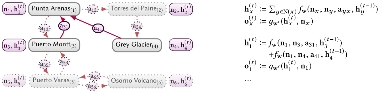
To illustrate, assume that we wish to identify new locations needing tourist information offices. In Figure 18, we illustrate the GNN architecture proposed by Scarselli and colleagues for a sub-graph of Figure 15, where we highlight the neighbourhood of ![]() In this graph, nodes are annotated with feature vectors (nx) and hidden states at step t (hx(t)), while edges are annotated with feature vectors (axy). Feature vectors for nodes may, for example, one-hot encode the type of node (City, Attraction, etc.), directly encode statistics such as the number of tourists visiting per year, and so on. Feature vectors for edges may, for example, one-hot encode the edge label (i.e., the type of transport), directly encode statistics such as the distance or number of tickets sold per year, and so on. Hidden states can be randomly initialised. The right-hand side of Figure 18 provides the GNN transition and output functions, where N(x) denotes the neighbouring nodes of x, fw(·) denotes the transition function with parameters w, and gw′(·) denotes the output function with parameters w′. An example is also provided for Punta Arenas (x = 1). These functions will be recursively applied until a fixpoint is reached. To train the network, we can label examples of places that already have tourist offices and places that do not have tourist offices. These labels may be taken from the
In this graph, nodes are annotated with feature vectors (nx) and hidden states at step t (hx(t)), while edges are annotated with feature vectors (axy). Feature vectors for nodes may, for example, one-hot encode the type of node (City, Attraction, etc.), directly encode statistics such as the number of tourists visiting per year, and so on. Feature vectors for edges may, for example, one-hot encode the edge label (i.e., the type of transport), directly encode statistics such as the distance or number of tickets sold per year, and so on. Hidden states can be randomly initialised. The right-hand side of Figure 18 provides the GNN transition and output functions, where N(x) denotes the neighbouring nodes of x, fw(·) denotes the transition function with parameters w, and gw′(·) denotes the output function with parameters w′. An example is also provided for Punta Arenas (x = 1). These functions will be recursively applied until a fixpoint is reached. To train the network, we can label examples of places that already have tourist offices and places that do not have tourist offices. These labels may be taken from the
knowledge graph or may be added manually. The GNN can then learn parameters w and w′ that give the expected output for the labelled examples, which can subsequently applied to label other nodes.
Convolutional Graph Neural Networks
Convolutional neural networks (CNNs) have gained a lot of attention, in particular, for machine learning tasks involving images. The core idea in the image setting is to apply small kernels (a.k.a. filters) over localised regions of an image using a convolution operator to extract features from that local region. When applied to all local regions, the convolution outputs a feature map of the image. Multiple kernels are typically applied, forming multiple convolutional layers. These kernels can be learned, given sufficient labelled examples.
Both GNNs and CNNs work over local regions of the input data: GNNs operate over a node and its neighbours in the graph, while (in the case of images) CNNs operate over a pixel and its neighbours in the image. Following this intuition, a number of convolutional graph neural networks (ConvGNNs) – a.k.a. graph convolutional networks (GCNs) – have been proposed, where the transition function is implemented by means of convolutions. A benefit of CNNs is that the same kernel can be applied over all the regions of an image, but this creates a challenge for ConvGNNs, since – unlike in the case of images, where pixels have a predictable number of neighbours – the neighbourhoods of different nodes in a graph can be diverse. Approaches to address these challenges involve working with spectral or spatial representations of graphs that induce a more regular structure from the graph. An alternative is to use an attention mechanism to learn the nodes whose features are most important to the current node.
Aside from architectural considerations, there are two main differences between RecGNNs and ConvGNNs. First, RecGNNs aggregate information from neighbours recursively up to a fixpoint, whereas ConvGNNs typically apply a fixed number of convolutional layers. Second, RecGNNs typically use the same function/parameters in uniform steps, while different convolutional layers of a ConvGNN can apply different kernels/weights at each distinct step.
Next part: (section 5.4): Inductive knowledge – Symbolic learning.
Header image source: Crow Intelligence, CC BY-NC-SA 4.0.
References:
- Hogan, A., Blomqvist, E., Cochez, M., d’Amato, C., Melo, G. D., Gutierrez, C., … & Zimmermann, A. (2021). Knowledge graphs. ACM Computing Surveys (CSUR), 54(4), 1-37. ↩
- Scarselli, F., Gori, M., Tsoi, A. C., Hagenbuchner, M., & Monfardini, G. (2008). The graph neural network model. IEEE transactions on neural networks, 20(1), 61-80. ↩