
The Mathematics of Modeling: Solving Differential Equations [Systems thinking & modelling series]
This is part 51 of a series of articles featuring the book Beyond Connecting the Dots, Modeling for Meaningful Results.
Given a differential equation or System Dynamics model specification, how do you go about determining the results of the model? This is typically referred to as “solving” the model. Since differential equation models and system dynamics models are essentially one and the same, the techniques used to solve differential equations can be directly applied to System Dynamics models. They are the techniques used by Insight Maker when you simulate any of the models in this series.
For most of the rest of this section, we use the differential equation terminology rather than System Dynamics terminology. We do so because it is more concise and more elegantly addresses the issues discussed in this section, and also because we want to familiarize you with its terminology and concepts. If you ever get lost, just refer to the System Dynamics to differential equation translation table.
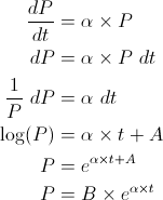
Let’s start our discussion of solving differential equations using our simple population model. As you recall, this model was:
![]()
![]()
What is the size of the population, at t = 10, given an α of 0.1? Calculus can be used to solve the model and answer this question. First we separate the terms of the derivative and integrate both sides of the equation. Thereafter it is a simple matter of algebra to solve for P:
Two new variables, A and B, appeared in this equation (where we arbitrarily set B = eA). These are unknown integration constants1. We can determine the values of the integration constants based on the initial conditions of the model, as we specified earlier that P(0) = 100. We evaluate the solution of the model at this initial condition to determine he value of B.
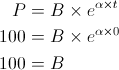
Thus our generic equation for P at any time and for any α is:
![]()
Plugging in α = 0.1 and t = 10, we obtain:
![]()
For this simple population model we have shown that we can obtain the precise population value at any point in the future. It took a fair amount of algebra even for such a simple model, but we did it!
Unfortunately, many differential equation models cannot be solved using these techniques. In practice, with most complex models it is impossible to analytically determine the values of the state variables in the future. This inability to solve a model can be true for even very simple models. Take for example the following growth model similar to our original one:
![]()
![]()
We have simply added a logarithm of P into our growth rate. Despite the smallness of this change, this model is now impossible to solve analytically. There is no analytic solution possible, but feel free to give it a try yourself (please don’t try too hard; we promise there is no solution). When developing complex models you should generally assume that no analytical solution will be available in practice. In cases like these, how can we go about developing solutions to the equations and determining the trajectory of the state variables in the system?
| Exercise 7-4 |
|---|
| Solve the differential equation:
|
| Exercise 7-5 |
|---|
| Solve the differential equation:
|
| Exercise 7-6 |
|---|
| Solve the differential equation:
|
The answer is numerical approximation. Even if we can’t solve the model equations analytically, we will always be able to approximate their results numerically. A number of different algorithms exist that allow us to approximate the solution to differential equations by repeatedly plugging values into them. To discuss these methods, it is useful to introduce some additional mathematical notation.
In our previous models, we have only looked at systems with a single state variable at a time. However, we can also consider systems containing multiple state variables. The Lotka-Volterra predator prey system we looked at earlier is an example of this. Given two populations of animals – let’s say a population of wolves (W) and a population of moose (M) – where the first population preys upon the second, we obtain a paired set of differential equations representing this predator-prey relationship:
![]()
![]()
When looking at algorithms to solve sets of equations like these numerically, it can be useful to denote y as a vector of all the state variables in the model. For the case of the exponential growth model y = [P] while for the Lotka-Volterra model y = [M, W]. When using this notation, yt indicates the vector of state variable values at a specific point in time, so y0 are the initial conditions for this model.
Additionally, we can denote y1 as the vector of derivatives for the different state variables. We treat these derivatives as functions of the current time and the values of the other state variables. To determine the rate of change of the state variables in a model at t = 10, we would write y1 (y10, 10) where y10 are the values of the state variables at t = 10.
The use of this notation might seem cumbersome, but it allows us to elegantly describe the mathematics of numerical solution algorithms without getting tied up in the details of a specific model.
Euler’s Method

The most basic numerical solution algorithm for differential equations is Euler’s method2. Simply put, assuming we know the state of the system at time t and we wish to estimate the state of the system at time t + Δt (where Δt is pronounced “delta-t” and represents the change in time) we can use the following equation:
![]()
Let’s walk through what this equation is doing. It first takes the derivatives for the state variables at the current point in time. It multiplies these rates of change by the Δt (how far in the future we want to know the results) and adds this change to the values of the state variables at the starting point in time. The result is an estimate of what the values in the future should be.
Let’s now apply this to a concrete example. Start with our population scenario, but instead of exponential growth we have a fixed inflow of people at a rate of 20 per year. At t = 0 we have 100 people and we want to know the population in 10 years. Using Euler’s method we obtain the following:
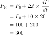
Thus the population size in 10 years will be 300. In this simple example, Euler’s method works perfectly and generates the exact same answer as we would have found using analytic solutions.
In general, however, we won’t be so lucky. For most problems Euler’s method will generate results that contain some level of error compared to what the true value should be. To see this let’s explore our exponential growth model again with an α of 0.1. As a reminder, this model is:
![]()
![]()
As we showed earlier, the precise solution to this model for t = 10 (to three decimal places) is 271.828. Let’s see what we get using Euler’s method with Δt = 10. Carrying out similar calculations as before we get:
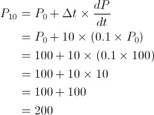
So using Euler’s method we obtain an estimate of 200 for the population size at t = 10 when we know the true value should be around 272. That’s a pretty large error! Why does this error occur? Why do we so significantly underestimate the final population size?
The reason is that we calculate the population’s rate of change only at t = 0. For each of the ten years we are simulating, we assume the population grows at the rate it would if there were exactly 100 people. However, the population size is constantly increasing during these ten years, so the rate at which it grows should also be increasing. Imagine the case of a bank account with an interest rate of 10% yearly. The bank account grows over time, so the interest earned should also grow from year to year. It’s the same principle of compounding here.
How do we address this issue? Using Euler’s method, we can do it simply by changing how often we calculate the rates of change. In our previous calculation, we went straight from t = 0 to t = 10 all in one step, using a Δt in Euler’s equation of 10. However, we could employ an alternate calculation strategy where, for instance, we stepped from t = 0 to t = 5, recalculated the derivative based on the new population size, and then stepped from t = 5 to t = 10. This would be equivalent to using a Δt of 5 and iterating the algorithm twice. Here is what we get doing this:
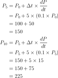
That result is certainly better, and we cut our error by over 33%. However, the error is still too large for most practical purposes. To improve the numerical estimation even more, we can apply smaller and smaller Δt’s. You probably have a good grasp of the calculations now, so let’s just show the results for each step of the simulation. We’ll look at Δt = 2 and Δt = 1.
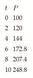

We see that as Δt gets smaller and smaller our results become more and more accurate. However, they are never perfect. There is always some error. Even if we made Δt as small as 0.1 (requiring 100 simulation steps), our final population size would be calculated to be 270, an error just under 1%.
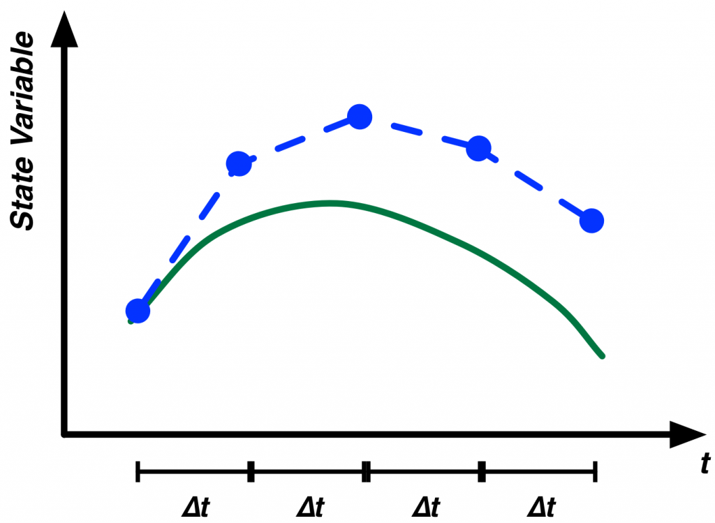
Figure 1 illustrates the application of Euler’s method to numerically estimate the trajectory for an example function. The smaller the Δt’s in the estimation, the better the results will be. Other terms that can be used in place of Δt are “Step Size”, “Time Step” or just “DT”. We prefer not to use the notation DT, as it can be easily confused with the dt from differential equations. The latter indicates an infinitesimally small change, while step sizes are never infinitesimally small.
As you decrease the step size for the simulation, the results of the simulation become more and more accurate3. The cost of this increased accuracy, however, is increased computation time. The computation time required by your model is directly proportional to 1 over the step size. Thus, if you cut the step size in half, your model will take twice as long to complete simulating.
In general, you want a step size small enough that your results are “accurate enough,” but one that isn’t so small that the simulation takes too long to complete. A rule of thumb for choosing the step size is to choose a starting step size that results in a fast simulation. Then cut the value of the step size in half and simulate the model again. If the results have not changed materially, keep the larger step size. If the results have changed, cut the step size in half again and repeat until the results cease to change.
| Exercise 7-7 |
|---|
| Take the differential equation:
|
| Exercise 7-8 |
|---|
| Take the differential equation:
|
Runge-Kutta Methods
Euler’s method is not the only technique that can be used to numerically solve differential equations. Other popular techniques are the Runge-Kutta methods. Runge-Kutta methods are a family of numerical differential equation solvers. In fact, Euler’s method itself can be classified as a simple Runge-Kutta method.
One widely-used member of the Runge-Kutta family of methods is a 4th-order Runge-Kutta method. This method differs from Euler’s method in that for each step, it evaluates the model multiple times and averages the resulting derivatives. Briefly, the driving set of equations for this method is as follows:
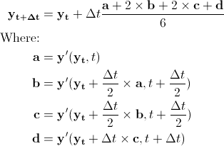
This algorithm first computes the derivatives of the system at the current time (a) and uses them to move the system forward to t + Δt/2. The derivatives are evaluated at t + Δt/2 (b) and this new set of derivatives is used to again move the system from t to t + Δt/2. A third set of derivatives is evaluated again at this mid-point (c) and used to move the system from t to t + Δt. A fourth set of derivatives is evaluated at this point (d). The system is then returned to its starting point and a weighted average of derivatives is used to move the system the full time step. This weighting puts most of the weight on the middle two derivatives instead of the derivatives from the end points.
This 4th-order Runge-Kutta method is generally much more accurate than Euler’s method for a given step size. Using a step size of 10 for our earlier population model, the Runge-Kutta method generates a value of 270.8. A step size of 5 yields a results of 271.7, just a smidgeon away from the precise value of 271.8. Recall that for Euler’s method, even with a step size of 0.1 we still were not as accurate as the Runge-Kutta method with a step size of 5. It is true that this 4th-Order Runge-Kutta method does a lot more work than Euler’s method for each step. It evaluates the model four times and has to do some averaging of derivatives. However, it is still much more accurate than Euler’s method for an equivalent level of computational effort.
| Exercise 7-9 |
|---|
| Take the differential equation:
Given a step size of 1, find the values of P at t = 0, 1, 2, 3, 4, 5 to one decimal place using the 4th-Order Runge-Kutta method. |
| Exercise 7-10 |
|---|
| Take the differential equation:
Given a step size of 1, find the values of P at t = 0, 1, 2, 3, 4, 5 to one decimal place using the 4th-Order Runge-Kutta method. |
| Exercise 7-11 |
|---|
| Discuss the differences between the 4th-Order Runge Kutta solutions and the Euler solutions. What causes these differences? Which method is most accurate? Why? |
| Exercise 7-12 |
|---|
| Describe a model where Euler’s method would be best suited as a numerical solver. Describe a model where the 4th-Order Runge-Kutta method would be best suited. |
A model exploring the selection of the simulation step size and differential equation solution algorithm can be found in Chapter 7 of Beyond Connecting the Dots.
Other Solution Techniques
This brief introduction into numerical solution methods for differential equations should enable you to intelligently make decisions about controlling the simulations of your models. It should help you identify potential sources of errors in your model and help you to adjust your simulation configuration to account for them.
The two methods we have looked at for solving differential equation models – Euler’s method and a 4th-Order Runge-Kutta method – are widely used and are built into Insight Maker. Many other methods are used in practice, and you should be aware of this richer ecosystem of solution techniques.
Although we do not have adequate space to delve into the full ecosystem of numerical differential equation algorithms, it is useful to briefly discuss one variant: the adaptive step size algorithm. The methods we have looked at here use a fixed step size specified at the beginning of a simulation. Many models, however, might be characterized by highly variable trajectories. One part of the trajectory might be very smooth and unchanging, while others might experience numerous rapid changes.
When using a fixed step size algorithm like the ones illustrated above, the step size must be set for the worse case scenario. The step size must be set to a small enough value to account for the rapidly changing areas. That said, the precision of this small step size is unnecessary on the smooth regions of the trajectory where the algorithm must do extra work for minimal gain in precision. Ideally, we would want to have a small step size for the rapidly changing areas and a large one for the smooth regions. This would result in the best of both worlds: high accuracy and quick computation.
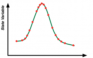
Adaptive step size algorithms do just that. They adjust the step size dynamically based on the behavior of the model’s derivatives. If the derivatives change rapidly, then the step size will automatically shrink; if the derivatives are constant or change very slowly the step size will automatically grow. Figure 2 illustrates the location of steps for an illustrative model using an adaptive step size algorithm. The steps are clustered around changes in the trajectory’s derivatives in an attempt to maximize predictive accuracy while minimizing computation effort.
Next edition: Equilibria and Stability Analysis: Introduction.
Article sources: Beyond Connecting the Dots, Insight Maker. Reproduced by permission.
Header image source: Beyond Connecting the Dots.
Notes:
- Recall from calculus that if A is a constant, then x2 + A dx = 2 × x. When we integrate 2 × x we need to add back in the constant term. We don’t know the value of this constant term immediately and we have to determine it later on. ↩
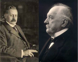
- Leonhard Euler was a brilliant 18th century Swiss mathematician who made many great advances in theoretical and applied mathematics. ↩
- It is important to note at this point that when we discuss accuracies in this context we are specifically referring to models comprising continuous differential equations. If you are using agent-based modeling or have discontinuities in your models – which could occur if you use If-Then-Else logic – then a smaller step size may not provide additional accuracy when there is some fundamental time step logic to the model. ↩


Is the differential equation in exercise 7-10 correct? It seems that Euler method quickly grows to infinite values.