
Optimization and Complexity: Finding the Best Fit [Systems thinking & modelling series]
This is part 62 of a series of articles featuring the book Beyond Connecting the Dots, Modeling for Meaningful Results.
After choosing how to measure a fit quantitatively, we need to find the set of parameter values that maximize the fit and minimize the error. To do this we use a computer algorithm called an optimizer that automatically experiments with many different combinations of parameter values to find the set of parameters that has the best fit.
Many optimizers start with an initial combination of parameter values and measure the error for that combination. The optimizer then slightly changes the parameter values in order to check the error at nearby combinations of parameter values. For instance, if you are optimizing one parameter, say the hamster birth rate, and your initial starting value is a birth rate of 20% per year; the optimizer will first measure the error at 20% and then measure the errors at 19% and 21%.
If one of the neighbors has a lower error than the initial starting point, the optimizer will keep testing additional values in that direction. It will steadily “move” toward the combination of parameters that results in the lowest error, one step at a time. If, however, the optimizer does not find any nearby combination of parameter values with a lower error than its current combination of parameter values, it will assume it has found the optimal combination of parameter values and stop searching for anything better.
The precise details of optimization algorithms are not important. You need to be aware of one key thing however: these algorithms are not perfect and they sometimes make mistakes. The root cause of these mistakes are so-called “local minimums”. An optimizer works by searching through combinations of different parameter values trying to find the combination that minimizes the error of the fit. The combination that has the smallest error is known as the true minimum or the “global” minimum.
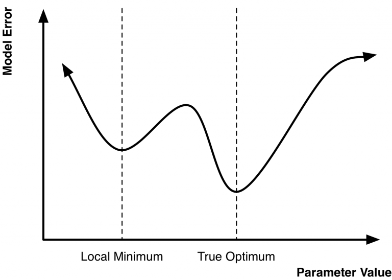
A local minimum is a combination of parameter values that is not the global minimum, yet whose nearby neighbors all have higher errors. Figure 1 illustrates the problem of local minimum. If the optimizer starts near the first minimum in this figure it might head toward that minimum without ever realizing that another, improved minimum exists. Thus, if you are not careful, you may think you have found the optimal set of parameters when in fact you have only found a local minimum that might have much worse error than the true minimum.
There is no foolproof way to deal with local minimums and no guarantee that you have found the true minimum1. The primary method for attempting to prevent an optimization from settling in on a local minimum is to introduce stochasticity into the optimization algorithm. Optimization techniques such as Simulated Annealing or Genetic Algorithms will sometimes choose combinations of parameter values at random that are actually worse than what the optimizer has already found. By occasionally moving in the “wrong” direction, away from the nearest local minimum, these optimization algorithms are more resilient and less likely to become stuck on a local minimum and more likely to keep searching for the global minimum.
Unfortunately, we have not been satisfied by the performance of these types of stochastic optimization algorithms. They are generally very slow and without fine-tuning by an expert can still easily become stuck in a local minimum. We prefer to use non-stochastic deterministic methods as the core of our optimizations. We then introduce stochasticity into the algorithm by using multiple random starting sets of parameter values. For instance, instead of carrying out a single optimization we will do 10 different optimizations, each starting at a different set of parameter values. If all 10 optimizations arrive at the same final minimum that is strong evidence we have found the global minimum. If they all arrive at different minima, then there is a good chance we have not found the global minimum.
A model illustrating the use of optimization and historical data to select the growth rate for a simulated population of hamsters can be found in Chapter 9 of Beyond Connecting the Dots.
| Exercise 9-5 |
|---|
| You are building a model to simulate company profits into the future. You will use 30 years of historical company profit data to calibrate parameter values using an optimizer.
Choose an error measure to use. Justify this choice and explain why you would use it instead of other measures. |
| Exercise 9-6 |
|---|
| Calculate the pseudo R2 for Growth Rate = 0.1, 0.3, and 0.172. |
| Exercise 9-7 |
|---|
| Adjust the JavaScript code to calculate pseudo R2 to use absolute value error instead of squared error. |
| Exercise 9-8 |
|---|
| Describe local minimum, why they cause issues for optimizers, and strategies for dealing with them. |
Next edition: Optimization and Complexity: The Cost of Complexity.
Article sources: Beyond Connecting the Dots, Insight Maker. Reproduced by permission.
Notes:
- This is true for the type of optimization problems you will generally be dealing with. Other types of optimization problems are much easier than the ones you may be encountering; they are known as convex optimization problems and are guaranteed not to have any local minimums. ↩