
Equilibria and Stability Analysis: Stability Analysis [Systems thinking & modelling series]
This is part 55 of a series of articles featuring the book Beyond Connecting the Dots, Modeling for Meaningful Results.
Now that we have learned how to analytically determine the location of equilibrium points, we may want to determine what type of stability occurs at these equilibria. As we stated earlier, for the incurable disease model it is trivial to conclude that the state of everyone being healthy is unstable, while the state of everyone being sick is stable. In more complex models, it may be harder to draw conclusions, or the stability of an equilibrium point may change as a function of the model’s parameter values. Fortunately, there is a general way to determine the precise stability nature of the equilibrium points analytically.
The procedure to do this is relatively straightforward, but the theory behind it can be difficult to understand. The first key principle that must be understood is that of “linearization”. To get a feel for linearization, let’s take the curve in Figure 1. Clearly this curve is not linear. It has lots of bends and does not look at all like a line.
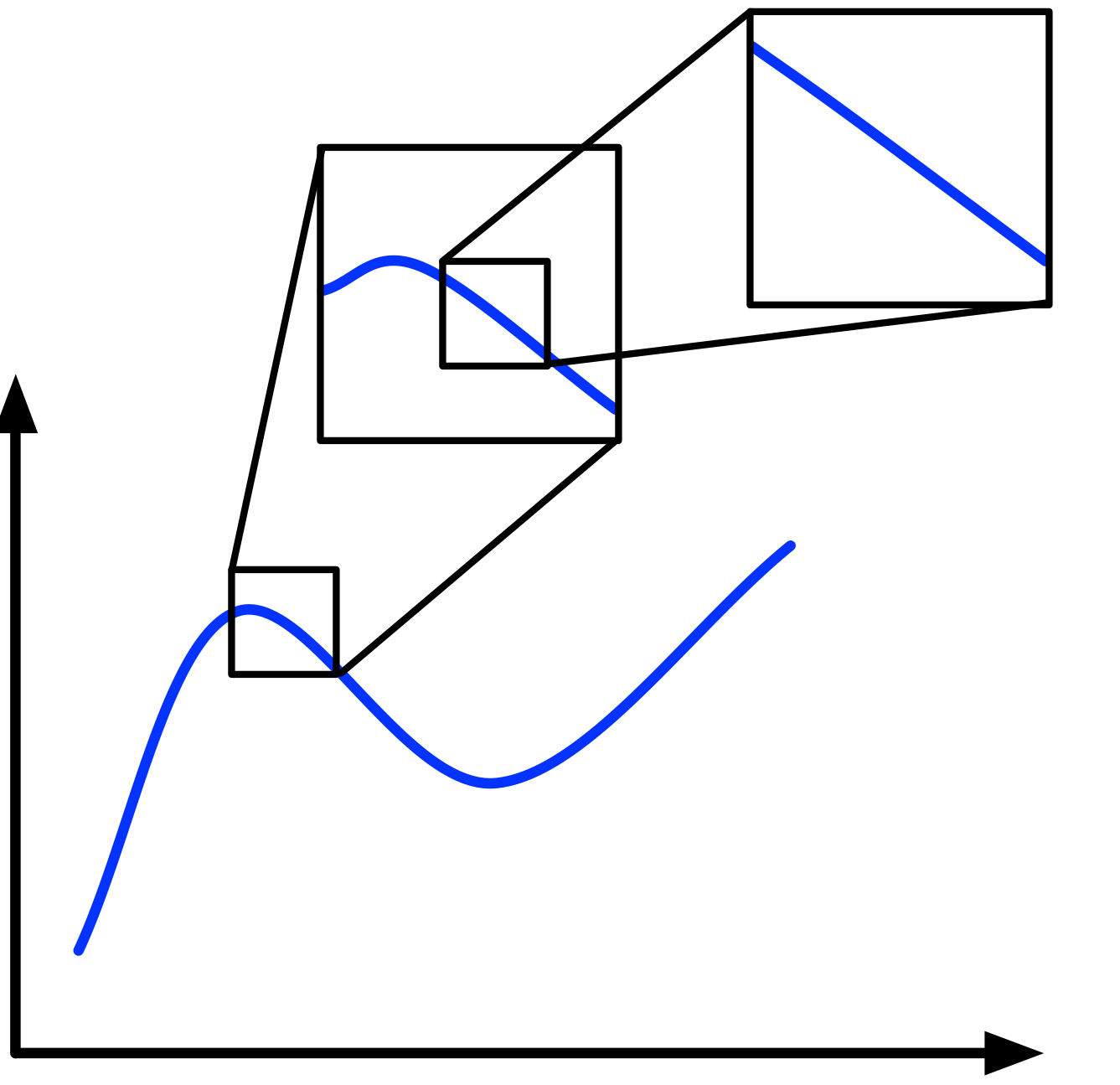
If we zoom in on any one part of the curve, however, the section we are zoomed in on starts to straighten out. If we keep zooming in, we will eventually reach a point where the section we are zoomed in on is effectively linear: basically a straight line. This is true for whatever part of the curve we zoom in on1. The more bendy parts of the curve will just take more zooming to convert them to a line.
We can conceptually do the same for the equilibrium points in our phase planes. Even if the trajectories of the state variables in the phase planes are very curvy, if we zoom in enough on the equilibrium points, the trajectories at a point will eventually become effectively linear. The simple, two-state variable exponential growth model we illustrated with phase planes above is an example of a fully linear model. If we zoom in sufficiently on the equilibrium points for most models, the phase planes for the zoomed-in version of the model will eventually start to look like one of these linear cases.
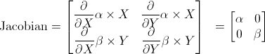
Mathematically, we apply linearization to an arbitrary model by first calculating what is called the Jacobian matrix of the model. The Jacobian matrix is the matrix of partial derivatives of each derivative in the model with respect to each of the state variables:

The Jacobian is a linear approximation of our (potentially) non-linear model derivatives. Let’s take the Jacobian matrix for the simple exponential growth model:

| Exercise 8-9 |
|---|
| Calculate the Jacobian matrix of the system:
|

| Exercise 8-10 |
|---|
| Calculate the Jacobian matrix of the system:
|

| Exercise 8-11 |
|---|
| Calculate the Jacobian matrix of the system:
|

This is complicated so don’t worry if you don’t completely understand it! Once you have the Jacobian, you calculate what are known as the eigenvalues of the Jacobian at the equilibrium points. This is also a bit complicated, so if your head is starting to spin, just skip forward in this section!
Nonetheless, eigenvalues and their sibling eigenvectors are an interesting subject. Given a square matrix (a matrix where the number of rows equals the number of columns), an eigenvector is a vector which, when multiplied by the matrix, results in the original vector multiplied by some factor. This factor is known as an eigenvalue and is usually denoted as λ. Given a matrix A, an eigenvalue λ with associated eigenvector B; the following equation will be true:
![]()
Let’s look at an example for a 2 × 2 matrix:
![]()
What eigenvector and eigenvalue combinations satisfy this equation? It turns out there are two key ones:
![]()
![]()
Naturally, any multiple of an eigenvector will also be an eigenvector. For instance, in the case above, [1, 0.5] and [-2, 2] are also eigenvectors of the matrix.
We can interpret eigenvectors geometrically. Looking at the 2 × 2 matrix case, we can think of a vector as representing a coordinate in a two-dimensional plane: [x,y]. When we multiply our 2 × 2 matrix by the point, we transform the point into another point in the two-dimensional plane. Due to the properties of eigenvectors, we know that when we transform an eigenvector, the transformed point will just be a multiple of the original point. Thus, when a point on an eigenvector of a matrix is transformed by that matrix, it will move inward or outward from the origin along the line defined by the eigenvector.
We can now relate the concept of eigenvalues and eigenvectors to our differential equation models. Take a look back at the phase planes for the exponential model example. For each phase plane, there are at least two straight lines of trajectories. The x- axis and the y-axis are the locations of these trajectories. A system on the x- or y-axis will remain on that axis as it changes. This indicates that for this model, the eigenvectors are the two axes, as a system on either of them does not change direction as it develops. That’s the definition of an eigenvector.
For our purposes though, we do not really care about the actual direction or angle for these eigenvectors. Rather, we care about whether the state variables move inward or outward along these vectors. We can determine this from the eigenvalues of the Jacobian matrix. If the eigenvalue for an eigenvector is negative, the values move inward along that eigenvector; if the eigenvalue is positive, the values move outward.
These eigenvalues tell us all we need to know about the stability of the system. Returning to our illustration of stability as a ball on a hill, we can think of eigenvalues as being the slopes of the hill around the equilibrium point. If the eigenvalues are negative, the ground slopes down towards the equilibrium point, forming a cup (leading to a stable equilibrium). If the eigenvalues are positive, the ground slopes away from the equilibrium point, creating a hill (leading to an unstable equilibrium).
Eigenvalues can be calculated straightforwardly for a given Jacobian matrix. Briefly, for the Jacobian matrix J, the eigenvalues λ are the values that satisfy the following equation, where det is the matrix determinant and I is the identity matrix.
![]()
We can do a quick example of calculating the eigenvalues for the Jacobian matrix we derived for our two-state variable exponential growth model.

That is a fair amount of work to do. It’s even more complicated if you have more than two state variables. However, once you have gone through the calculations and determined the linearized eigenvalues for your equilibrium points, you know everything you might want to know about the stability of the system.
| Exercise 8-12 |
|---|
| Find the eigenvalues of the following matrix:
|
| Exercise 8-13 |
|---|
| Find the eigenvalues of the following matrix:
(Bonus: Determine the associated eigenvectors.) |
| Exercise 8-14 |
|---|
| Find the eigenvalues of the following matrix:
(Bonus: Determine the associated eigenvectors.) |
| Exercise 8-15 |
|---|
| Find the eigenvalues of the following matrix:
(Bonus: Determine the associated eigenvectors.) |
In the exponential growth model we can see that when the eigenvalues are both negative we have a stable equilibrium (refer to the graphs we developed earlier), while if either one is positive (or they both are) we have an unstable equilibrium. This is logical, since if either one is positive it pushes the system away from the equilibrium, making it unstable. If they are both negative, they both push the system toward the equilibrium point. Visualize the ball sitting in the cup or on the hill.
Looking at it this way, we realize that all we need in order to understand the stability of an equilibrium point are the eigenvalues of the Jacobian at the equilibrium point. This is an incredibly powerful tool. It reduces the complex concept of stability into an analytical procedure that can be applied straightforwardly.
Let’s now look at some more examples.
First let’s take our simple disease model from earlier. If you recall, that model was:

First let’s calculate the Jacobian for this model. We take the partial derivatives of the two derivatives with respect to each of the two state variables to create a two-by-two matrix:

Next, we evaluate this Jacobian at one of our equilibrium points. Let’s choose the one where the S = 0 (no one is sick) and H = P (where P is the population size) so everyone is healthy:
![]()
We can now find the eigenvalues for this matrix. Once we go through the math we get two eigenvalues: 0 and α × P. What do these mean? Well, since one of the eigenvalues is positive, this indicates we have movement away from the equilibrium point along at least one of the eigenvectors. The other vector has no movement (0 as the eigenvalue), but this one positive value will ensure we have an unstable equilibrium. Again, think of the ball. The positive eigenvalue indicates the ground slopes downward from the equilibrium point so a ball balanced on top of this hill will be very unstable.
Now let’s do the second equilibrium – the one where S = P and H = 0 (everyone is sick). Let’s evaluate the Jacobian at this equilibrium:
![]()
Now let’s find the eigenvalues for this matrix. Once we go through the math we get two eigenvalues: this time 0 and −α × P. Again, the 0 eigenvalue can be ignored, as it does not cause growth or change. However, the second eigenvalue is negative, indicating the system moves toward the equilibrium point again. Look back at our exponential growth phase planes. Negative coefficients indicate trajectories towards the equilibrium (create a cup for the ball). Thus, this second equilibrium is a stable one.
You can see this is a very powerful tool. The following table summarizes the types of eigenvalues that can be found for a system with two state variables and their associated stabilities. In this table, “damped” oscillations refers to a system that oscillates around a point of stability. Over time, the oscillations will “dampen” growing smaller and smaller in size until the system arrives at the point of stability.
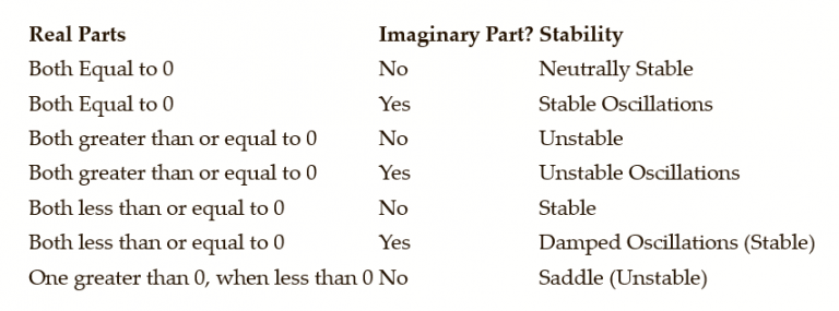
A “saddle” point is a point where one eigenvalue is positive and the other one is negative. In this case, one eigenvalue pushes the system towards stability, and the other eigenvalue pushes the system away from stability. The net effect of this process is actually instability. Only a single eigenvalue pushing the system away from stability is enough to make the system unstable.
| Exercise 8-16 |
|---|
A system’s Jacobian matrix has two eigenvalues at an equilibrium point. Determine the stability of the system at this point for the following pairs of eigenvalues:
|
| Exercise 8-17 |
|---|
A system’s Jacobian matrix has two eigenvalues at an equilibrium point. Determine the stability of the system at this point for the following pairs of eigenvalues:
|
| Exercise 8-18 |
|---|
A system’s Jacobian matrix has a single eigenvalue at an equilibrium point. Determine the stability of the system at this point for the following eigenvalues:
|
Next edition: Equilibria and Stability Analysis: Analytical vs. Numerical Analysis.
Article sources: Beyond Connecting the Dots, Insight Maker. Reproduced by permission.
Header image source: Beyond Connecting the Dots.
Notes:
- The one exception to this rule is if your curve is some sort of fractal. In this case no matter how much you zoom in on it, the curve will never become straight. In practice, however, this caveat is a non-issue. ↩