The Mathematics of Modeling: Differential Equations and System Dynamics [Systems thinking & modelling series]
This is part 50 of a series of articles featuring the book Beyond Connecting the Dots, Modeling for Meaningful Results.
This section places the modeling techniques introduced earlier in this interactive learning environment (ILE) within a firm mathematical framework. The contents of this chapter are quite technical, and to fully understand them requires knowledge of basic calculus and linear algebra. We present the material because it is important both for readers who want a deep understanding of how their models operate and those who wish to understand how System Dynamics fits within the larger field of mathematical modeling. Users who approach systems thinking and modeling from a more qualitative angle may browse or safely skip this material.
Differential Equations and System Dynamics
Differential equations are a common mathematical tools used to study rates of change. Some basic terminology needs to be learned in order to discuss differential equations. We will introduce this new terminology and then tie it back to the modeling techniques you’ve already learned.
State Variable: A state variable is an object that represents part of the state of a system. For instance, in a population model you could have a state variable representing the current number of individuals in that population. In a model of a lake, you could have a state variable representing the current volume of water in the lake. In equations, state variables are often represented using Roman letters such as X, Y or Z.
Derivative: Derivatives define rates of change in state variables. For instance, if we had a state variable representing the size of a population, a derivative would specify how this population grows or shrinks over time. The population’s derivative would aggregate all changes such as births, deaths, and immigration or emigration to show the net change in the state variable over time. Similarly, in the case of a model of a lake, the lake volume state variable would have a derivative showing how much net water flows into or out of the lake over time. Given a state variable X, the derivative of X with respect to time is generally written as dX / dt but can also be written as X’ or Ẋ.
Let’s put this new terminology to work to define a simple model. We start by creating an exponential growth population model. We only need one state variable in this model to represent the size of the population. We denote this state variable as P. We need to define one parameter to control the growth rate in the population. We will denote this growth rate parameter α.
The resulting differential equation exponential growth model can be written simply as:
![]()
This indicates that the rate of change for the population for one unit of time is α × P. Our model is not quite fully specified yet, as we do not know what the initial value of the population is. Differential equation models are often additionally specified by providing the values of the state variables at a specific point in time. Below we indicate that the population size at time 0 is 100.
![]()
![]()
You may have already noted that this model is easy to construct using the techniques we have already introduced. In fact, we have discussed this type of model several times. We could construct it with System Dynamics tools using a stock to represent the population (P), a flow to represent the change of population (dP / dt), and a variable to represent birth rate (α). We could specify our initial condition of a population size of 100 by setting the initial value for the stock for 100.
This is an important point. Many differential equation models1 can be directly represented using the System Dynamics modeling techniques described in this series. Similarly, a System Dynamics model can be rewritten as a differential equation model.
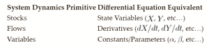
From this perspective, System Dynamics models and differential equation modeling are one and the same. A System Dynamics model can be expressed using differential equation notation and vice versa. To see this in more detail, we can look at the mapping between System Dynamics and differential equation models. There is a one-to-one direct correspondence between the key System Dynamics primitives and components of a differential equation model.
Since they do not differ significantly from a mathematical standpoint, what separates these two approaches to modeling? Where System Dynamics and differential equation modeling differ is in their focus and philosophy. The primary goal for differential equation modelers is analytic tractability (in other words, how easy is it to mathematically manipulate and understand the model’s equations?). This analytic tractability allows these modelers to derive definite results and conclusions from the model’s equations. System Dynamics modelers generally are less concerned about analytic tractability and are more comfortable with simulating the model and drawing conclusions from observed trajectories and numerical results.
To go further, System Dynamics modelers care greatly about communicating their models, deliberately mirroring reality to some extent and exploring the consequences of feedback. The differing focuses on communication between System Dynamics modelers and differential equation modelers can be seen in the method of naming variables. Differential equation models are generally dominated by abstract Greek symbols (e.g. α) while System Dynamics models generally clearly spell out variable names (e.g., “Birth Rate”) and additionally use a model diagram to illustrate and communicate the relationships among different parts of the model.
| Exercise 7-1 |
|---|
| You have a System Dynamics model simulating water leaking out of a hole in a jar. You have a stock Jar with an initial value of 40. Roughly 10% of the water leaks out of the jar every time period and there is a single flow leading out of the jar with the rate 0.10*[Jar]. Express this model using differential equations. |
| Exercise 7-2 |
|---|
| You have a System Dynamics model simulating people becoming sick. You have two stocks in the model Healthy and Infected. There is a single flow, Infection, going from the healthy to infected stock with a flow rate of 0.05*[Infected]*[Healthy]. Initially there are 100 healthy people and 1 infected person. Express this model using differential equations. |
| Exercise 7-3 |
|---|
| You have a differential equation model of an animal population’s growth (denoted P). The population growth is parameterized by the parameter r and a maximum population size or carrying capacity of K. The following differential equations define this model:
Implement a System Dynamics version of this model. What is the size of the population after 100 years? |

Next edition: The Mathematics of Modeling: Solving Differential Equations.
Article sources: Beyond Connecting the Dots, Insight Maker. Reproduced by permission.
Header image source: Beyond Connecting the Dots.
Notes:
- Specifically those where the denominator in the dX / dt derivative is always dt: a very wide class of commonly used models. ↩
I tend to disagree with your statements somewhat:
Typically, a model representation, say in computer science, is done in a way that is agnostic to the method of solution, e.g., in an ordinary differential equation model dt or TIME STEP cannot be used within equations. Specifying dt should be open to the solver used eventually and equations are formulated with continuous time in mind.
This is clearly not the case in system dynamics, where TIME STEP and fixed step solution methods are rather “hard wired” into the model equations, which typically are formulated with the explicit, fixed-step Euler method in mind. Most system dynamics tools cannot deal with time or state events, i.e., “events” can only happen at multiples of the TIME STEP and typically will take up time, e.g., the effect is not instantaneous but takes a TIME STEP.
Another difference would be that most of the software I am aware of uses assignments ( left hand side := right hand side), not equations. This later typically requires modern differential algebraic equation (DAE) solvers.
System Dynamics looks more like difference equations to me where instead of x(t+1) = f(…) x(t + dt) = f(…) is written. This is decidedly different from truly writing equations in discrete time. Note, that simulation languages like Modelica allow to combine true continuous-time differential equation modeling with graphical (structural) modeling and also allow for longer variable names. 😉