Building Confidence in Models: Model Results [Systems thinking & modelling series]
This is part 42 of a series of articles featuring the book Beyond Connecting the Dots, Modeling for Meaningful Results.
Assuming the design of the model and its implementation are correct, the modeler must still transfer confidence in the model’s results to its audience. This can be done in several different ways.
Expected Results
The first way is to demonstrate that the model generates expected results for normal inputs. For instance, if you modeled a reservoir, you would expect the volume of the reservoir to decline during the summer due to evaporation if no more water flowed into it. You can also test extreme scenarios and show that they generate the expected results. For example, if your reservoir were empty, you would expect the amount of water evaporating from it to be zero. By enumerating these standard cases and showing that the model results match the expected results you can help build confidence in the model.
Often these expected results can be described in terms of a curve showing how the values of one of the stocks (or variables) in the system is expected to change over time. This curve can be taken from historical data (a reference behavior pattern), or simply drawn on a piece of paper by experts familiar with the system (an excepted behavior pattern).
Counter-intuitive Results
Another way to increase confidence in a model is to show unexpected, but justifiable, results. Imagine a model that for a certain set of inputs would create what, at first glance, appeared to be the “wrong” behavior. Some lever in the model could lead to unexpected results. When first shown these results, an audience could have low confidence in the model. If the audience was then walked through the model step by step to show how those results were correct and mirrored reality, that could well increase their confidence in the model results.
Forecasting
Possibly the most persuasive action to convince an audience of the effectiveness of a model is to forecast the future and then show this forecast to be correct. This, of course, is difficult to do in practice for several reasons. Depending on the scale of a model, it could take several years or decades to generate data to test the model. Additionally, we must remember that most narrative models are poor predictors and should not be used for predictive purposes solely.
Sensitivity Testing
Sensitivity testing is a broad field that has the potential to address many questions and doubts that may arise about a model. In general, the variables and numeric configuration values in a model will never be known with complete certainty. When the results from an election poll are published, the pollsters publish not only their predictions but also the uncertainty in the prediction (e.g., “the Democratic candidate will obtain 52% ± 3% of the vote”). Similarly, when a building is constructed, the materials used will have certain properties – such as strength – that again are only known up to some error or tolerance. The engineer and contractor are responsible for ensuring that the materials are sufficient even given the uncertainty of their exact strengths.
The same occurs when modeling. The modeler will have to estimate most primitive values, along with associated errors. Of course the error will also be propagated through the model when it is simulated, and will affect the results generated by the model. This error is one factor that can create doubt about a model and reduce an audience’s level of confidence.
As a modeler, one approach to address doubt would be to try to measure all the model’s variables with great accuracy. You could search the available literature, undertake a meta-analysis of current results, carry out new experiments, and survey experts to get as precise a set of parameter values as possible. If you were able to say with strong certainty that these values were so accurate and the errors so small that their effect on the results is negligible, then that would be one way of addressing the issue of uncertainty.
However, all of this is often impossible to do. When dealing with complex systems it is almost always the case that at least a couple variable values will never be known fully with certainty. No matter how much research you do or how many experiments you perform, you will never be able to pin down the precise values of these variables. How do we handle these cases?
The answer is straightforward: Rather than trying to eliminate the uncertainty, we embrace it by explicitly including it in the model. If you can then show that the results of your model do not significantly change, even given the uncertainty, you have a persuasive case for the validity of your results. Of course the results will always change when the uncertainty is introduced, but if the conclusions persist even in the face of this uncertainty, the audience will be more confident in the model and its results.
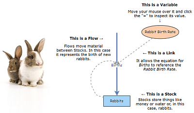
Uncertainty can be explicitly integrated into a model by replacing constant primitive values with a construct that represents the uncertainty in that value. Imagine you had a simple population model of rabbits in a cage. You want to know how many rabbits you will have after two years. However, you don’t know how many rabbits there are in the cage initially. You have been told that there are probably 12 rabbits, but the true number could range anywhere from 6 to 18.
If you model your population as a single stock, what should the initial value be? A naive model could be built where you specify the initial value of the rabbit stock as 12. However, that does not incorporate the uncertainty and could be a source of criticism or doubt for the model. An alternative would be to specify that the initial value of the stock is a random number with a minimum value of 6 and a maximum value of 18. So each time you run the model you will get a different result. If you ran the model once, the initial value might be chosen to be 7 and you would obtain one result. If you ran the model again, the initial value might be 13 and you would get a different result.
If you run this stochastic model many times, you obtain a range of results. These results can be automatically aggregated to show the range of outputs. For instance, if you ran the model 100 times you could see what the maximum and minimum final populations were. This would give you a good feeling for how many rabbits you needed to prepare for after two years. In addition to the maximum and minimum you might be interested in the average of these 100 runs: the expected number of rabbits you would see. You could also plot the distribution of the final population sizes using a histogram to see how the results are distributed. This distribution would show how sensitive the outputs are to the uncertainty in the inputs: a form of sensitivity testing.
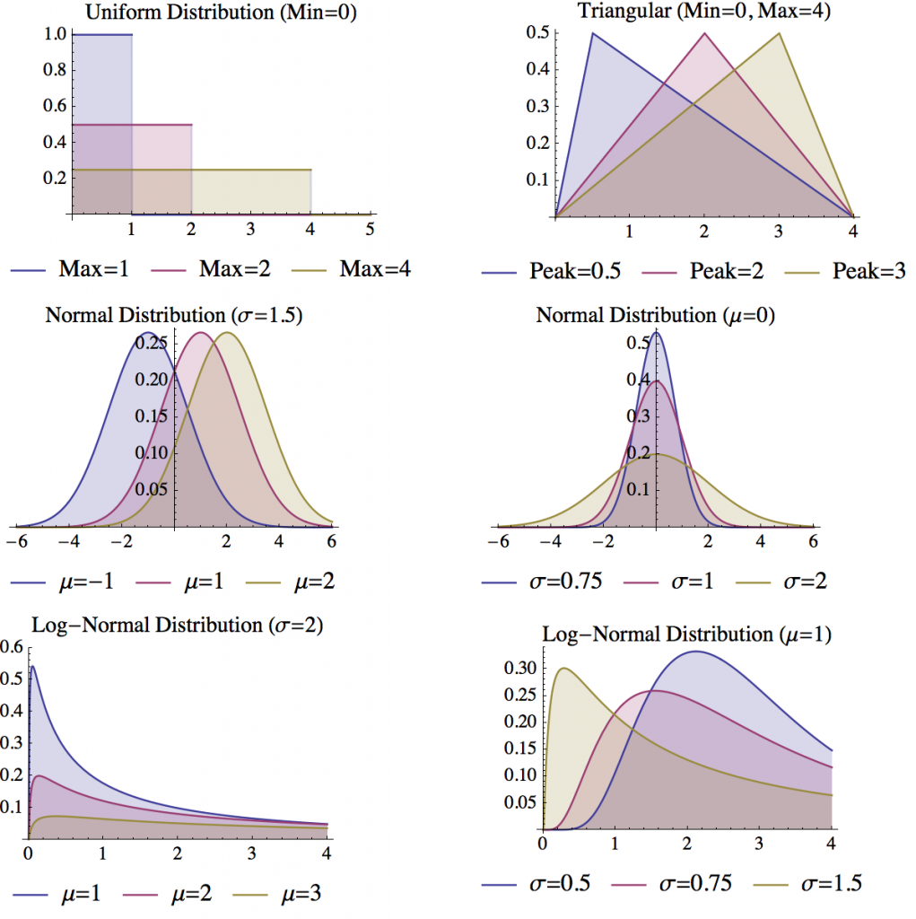
Four key distributions are useful for specifying the uncertainty in a variable:
- Uniform Distribution: The uniform distribution is defined by two parameters: a minimum and a maximum. Each number within these boundaries has an equal probability of being sampled. The uniform distribution is useful when you know the boundaries on the values a variable can take on, but you do not have any information on the likelihood of the different values within this region. The uniform distribution can be used in Insight Maker using the function Rand(Minimum, Maximum), the two parameters are optional and will default to 0 and 1 if Rand() is called without them.
- Triangular Distribution: The triangular distribution is defined by three parameters: the minimum, the maximum, and the peak. Like the uniform distribution, the triangular distribution will only generate numbers between the minimum and maximum. Unlike the uniform distribution, the triangular distribution will not sample all numbers between these boundaries with equal likelihood. The value specified by the peak will have the most likelihood of being sampled, with the likelihood falling off as you move away from the peak towards either the minimum or maximum boundary. The triangular distribution is useful when you know both the most likely value for a variable and the boundaries for the values a variable can take on. The triangular distribution can be used in Insight Maker using the function RandTriangular(Minimum, Maximum, Peak).
- Normal Distribution: The normal distribution is defined by two parameters: the mean of the distribution (generally denoted μ) and the standard deviation of the distribution (generally denoted σ). The most likely value to be sampled from the normal distribution is the mean. As you move away from the mean (in either a positive or negative direction), the likelihood of a number being sampled decreases. The standard deviation controls how fast this likelihood falls as you move away from the mean. Small standard deviations result in steep declines in the likelihood, while large standard deviations result in more gradual declines. The normal distribution is useful when you do not have boundaries on the values for a variable but you know what the most likely value for the variable should be (the mean). The normal distribution can be used in Insight Maker using the function RandNormal(Mean, Standard Deviation).
- Log-normal Distribution: The log-normal distribution is closely related to the normal distribution. In fact, the logarithm of the values samples from a normal distribution will be log-normally distributed. Like the normal distribution, the log-normal distribution is defined by two parameters: the mean and standard deviation. The log-normal distribution differs from the normal distribution in that negative values will never be generated by the log-normal distribution. Thus it is useful when you have a variable which you know cannot be negative but for which you do not have an upper bound. The log-normal distribution can be used in Insight Maker using the function RandLogNormal(Mean, Standard Deviation). The log-normal distribution can also be used to represent other types of one-sided boundaries. For instance, the following equation could be used to represent a variable whose number was always less than 5: 5–RandLogNormal(2, 1)
There are many other forms of probability distributions. Some notable ones are the Binomial Distribution (RandBinomial(Count, Probability)), the Negative Binomial Distribution (RandNegativeBinomial(Successes, Probability)), the Poisson Distribution (RandPoisson(Lambda)), the Exponential Distribution (RandExp(Lambda)) and the Gamma Distribution (RandGamma(Alpha, Beta)). These distributions can be used to address very specific modeling use cases and needs (for instance, the Poisson distribution can be used to model the number of arrivals over time), however, the four distributions described in detail above should generally be sufficient for most sensitivity testing needs.
An important practical tip when using sensitivity testing within the System Dynamics context is to be careful about specifying random numbers within variables. The value of a variable is recalculated each time step. This means that if you have a random number function in the variable, a new random value will be chosen each time step. This can create a problem if the random value is supposed to be fixed across the course of the simulation. For instance, we may not know the birth rate coefficient for our rabbit population, but, whatever it is, we assume it is fixed over the simulation.
A simple way to handle these fixed variable values would be to replace the variables with stocks. The initial value for the stocks could be set to the random value; it would only be evaluated once at the beginning of the simulation and kept fixed thereafter. Though very workable, this approach violates the fundamental metaphors at the heart of System Dynamics. In Insight Maker, another approach is to use the Fix() function. When used with one argument, this function evaluates whatever argument is passed to it a single time, and then returns the results of that initial calculation for subsequent time steps. So instead of having the simple equation Rand(0, 10) in a variable to generate a random number between 0 and 10, you could place Fix(Rand(0, 10)) in the variable. The first equation would generate a new random number each time step; the second equation will generate one random number and keep it constant throughout the simulation.
This model helps you explore the usage of sensitivity testing in practice.
Need help? See the Model instructions
| Exercise 5-2 |
|---|
| Create an equation to represent the uncertainty of how many red marbles there are in a bag. You know there are at least 5 red marbles and no more that 14. You do not have any other information. |
| Exercise 5-3 |
|---|
| Create an equation to represent the uncertainty of how many red marbles there are in a bag. You know there are probably about 20 red marbles and you know there are no more than 100 marbles in the bag. |
| Exercise 5-4 |
|---|
| Create an equation to represent the uncertainty of how many red marbles there are in a bag. You know there are probably about 20 red marbles and you do not know how many marbles the bag can hold total. |
The astute reader will notice that our discussion up to this has failed to address an important point: how do we determine the uncertainty of a variable? It is very easy to say that we do not know the precise value of a variable, but it is much more difficult to define the uncertainty of it. One case where we can precisely define uncertainty is when we take a random sample of measurements. For instance, suppose our model included the height of the average American man as a variable. We could randomly select a hundred men and measure their heights. In this case our uncertainty would be normally distributed with a mean equal to the mean of our sample of one hundred men and a standard deviation equal to the standard error of our sample of one hundred men1. For any random sample of n values from a population, the same should hold true: you will be able to model your uncertainty using a normal distribution with:
![]()

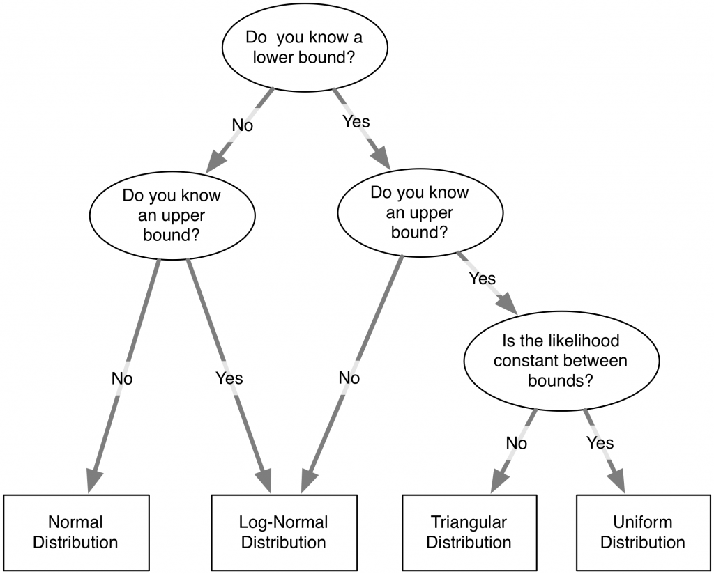
However, in most applied cases you will not be able to apply this normality assumption. Generally you will not have a nice random sample, or you might have no data at all and instead have some abstract variable for which you need to specify a value. In these cases, it is up to you to make a judgment call on the uncertainty. Choose one of the four distributions detailed above and use the expert knowledge available to you to place an estimate on the parameterization of uncertainty. One rule of thumb: it is better to overestimate uncertainty than underestimate it. It is better to err on the side of overestimating your lack of knowledge than it is to obtain undue confidence in model results due to an underestimation of uncertainty.
| Exercise 5-5 |
|---|
| You have tested the diameter of 15 widgets coming out of a factory and obtained the following values: 2.3, 2.5, 1.9, 1.4, 2.0, 2.7, 1.9, 2.1, 2.1, 2.2, 1.6, 2.4, 2.0, 1.8, 2.6.
Create an equation to generate a new widget size with the same distribution as the widgets arriving from the factory. |
| Exercise 5-6 |
|---|
| You have taken 12 sheep from a population and weighed the amount of wool on each sheep to obtain the following weights in kilograms: 1.005, 0.817, 0.756, 0.821, 0.9, 0.962, 0.692, 0.976, 0.721, 0.828, 0.718, 0.852.
Create an equation to generate a random variable for how much wool you will obtain from a sheep. |
Next edition: Building Confidence in Models: Confidence and Philosophy.
Article sources: Beyond Connecting the Dots, Insight Maker. Reproduced by permission.
Header image source: Beyond Connecting the Dots.
Notes:
- Please note that this contradicts slightly what we said earlier. Clearly, a person cannot have a negative height while the normal distribution will sometimes generate negative values. So wouldn’t a log-normal distribution be better than a normal distribution? Mechanistically, it would, however statistically we can show that due to the Central Limit Theorem the normal distribution does asymptotically precisely model our uncertainty. Given a large enough sample size (100 is more than enough in this case), the standard deviations for uncertainty will be so small that the chances of seeing a negative number (or even one far from the mean) are effectively none. ↩

